Introduction
This article describes creating the Adverse Events Tornado Plot
for Oncology Studies. It can be used for the reports
adae_tornado.tot; as well as for CDISC-recommended Tornado Plot.
Examples are created using in-built ADAE and
ADSL dataset.
Programming Flow
Process Data with Subsets and Variables
Before creating Adverse Events tornado plot, it’s
essential to use the process_tornado_data(). This function
helps prepare the data for visualization, making it a crucial step. With
this function, users can customize many parts of the plot to match their
specific data and analysis needs.
While it is recommended that this be used for Oncology data, it can also
work with non-Therapeutic Area specific ADaM datasets, which is shown in
this example.
This function block consists mainly adsl_merge(),
ae_pre_processor() and mentry() functions to
combine ADSL variables, perform adverse-event specific pre-processing
and filter records/set grouping variables. It also filters out the
maximum severity based on the given inputs. Below, we’ll explain the
parameters used in process_tornado_data:-
dataset_adsl: This parameter is used to pass the variable containingADSLdataset.dataset_analysis: This parameter is used to pass the variable containing analysis dataset. In this example,ADAEdataset.adsl_subset: This parameter specifies subset condition(s) for theADSLdataset. It allows the user to filter data before plotting.analysis_subset: Similar toadsl_subset, this parameter specifies subset condition(s) for the analysis dataset.split_by: This parameter is used for splitting the data by a specific variable. The default value isNA_character_which suggests that by default, there’s no splitting. If a variable is provided, it would split the data accordingly. Example: Region - separate plots would be generated for each region.trtvar: This parameter represents the treatment variable. It indicates the variable that represents different treatments or groups in the data.trt_left: This parameter represents the treatment value. It indicates the value that displays on the left hand side of the plot.trt_right: This parameter represents the treatment value. It indicates the value that displays on the right hand side of the plot.trtsort: This parameter is used for sorting the treatment variable.obs_residual: This parameter is used to pass a period (numeric) to extend the observation period. If passed as NA, overall study duration is considered for analysis. eg. if 5, only events occurring upto 5 days past the TRTEDT are considered..fmq_data: This parameter is required if FMQ terms are to be used as high or low terms, theFMQ_Consolidated_Listshould be passed. Default value isNULL.ae_catvar: This parameter is used for series categorical variable for severity analysis and filter out the maximum severity.denom_subset: This parameter is a condition which is used to subset data set for calculating denominator. Default value isNA.pctdisp: This parameter is a method that is used to calculate denominator (for %). Valid values:"TRT","VAR","COL","SUBGRP","CAT","NONE","NO","DPTVAR","BYVARxyN".legendbign: This parameter determines whetherNshould be displayed in the legend. The default value isYwhich suggests that by default,Nis displayed in legend. Default value isN.yvar: This parameter represents the variable to be plotted on the y-axis. The default value isAESOC.
NOTE: Default/Example values are provided to give users a starting point. However, these values can be modified as necessary to better suit the specific data and visualization objectives.
The first step for creating tornado_plot for Adverse
Events is to read the required datasets into the environment. In this
example, ADSL and ADAE are used.
Below is an example of calling process_tornado_data
function for preprocessing the data for tornado plot.
df <- process_tornado_data(
  dataset_adsl = adsl,
  dataset_analysis = adae,
  adsl_subset = "SAFFL == 'Y'",
  analysis_subset = "TRTEMFL == 'Y'",
  obs_residual = "30",
  fmq_data = NA,
  ae_catvar = "AESEV/AESEVN",
  trtvar = "ARM",
  trt_left = "Xanomeline High Dose",
  trt_right = "Xanomeline Low Dose",
  pctdisp = "TRT",
  denom_subset = NA_character_,
  legendbign = "N",
  yvar = "AESOC"
)
The process_tornado_data returns data.frame
which gets stored in df above. A pre-processed dataset
which is the input for Oncology tornado plot.
df
Tornado Plot
The tornado_plot function is designed to create flipped
bar plots from input data, with customizable options. It offers
flexibility in plotting data and allows users to tailor the plot
aesthetics to their preferences. The parameters used in
tornado_plot are explained below:
datain: The input data for plotting. The output data from process_tornado_data function.trt_left_label: This parameter is used to label thetrt_leftin the plot.trt_right_label: This parameter is used to label thetrt_rightin the plot..bar_width: Bar width option. This parameter allows customization of the bar width displayed on the plot.axis_opts: List of options for axis appearance. This parameter allows customization of the appearance of the x-axis and y-axis, including labels, and other options retrieved from plot_axis_opts().legend_opts: List of options for legend appearance. This parameter allows customization of the legend displayed on the plot, including its label, position, and direction.series_opts: Vector of color options with namedae_catvarvariable for the severity analysis.griddisplay: Grid display option. This parameter controls whether grid lines are displayed on the plot. Set it to “N” to disable grid lines, and “Y” to enable them.
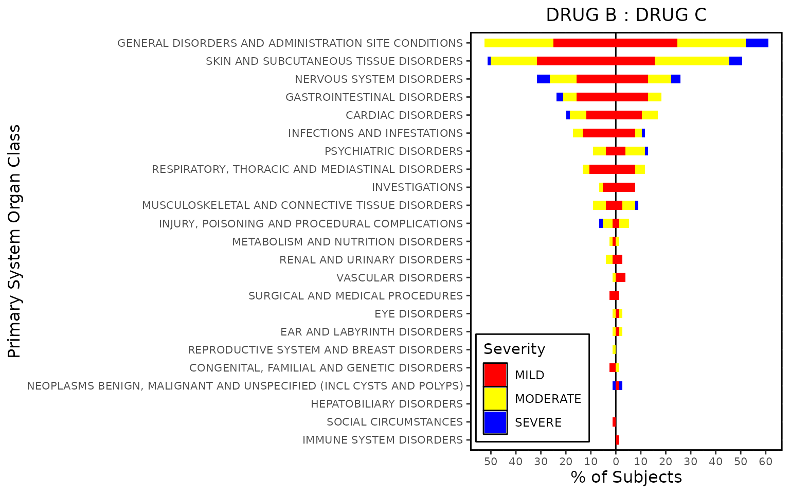
Below is an example of how oncology tornado plot is
called using the defined parameters:
series_opts <- g_seriescol(df, "red~yellow~blue", "BYVAR1")

plot <- tornado_plot(
  df,
  trt_left_label = "DRUG B",
  trt_right_label = "DRUG C",
  bar_width = 0.5,
  axis_opts = plot_axis_opts(
    xaxis_label = "Primary System Organ Class",
    yaxis_label = "% of Subjects",
    ylinearopts = list(
      breaks = seq(-100, 100, 10),
      labels = c(seq(100, 0, -10), seq(10, 100, 10))
    )
  ),
  legend_opts = list(
    label = "Severity",
    pos = c(0.2, 0.15),
    dir = "vertical"
  ),
  series_opts = series_opts,
  griddisplay = "N"
)
print(plot)